
Newsletter
Suscríbete a nuestro Newsletter y entérate de las últimas novedades.
https://centrocompetencia.com/wp-content/themes/Ceco
volver
Broadly speaking, elasticity serves as a quantitative measure of the sensitivity of one variable to fluctuations in another. In economics, elasticity () is mainly used to measure how much buyers and sellers react to changes in market conditions (Mankiw, 1997).
The generic formula to calculate elasticities of demand or supply in relation to price is:
\epsilon = \frac{\Delta \% Q}{\Delta \% P}
Here, “ \Delta \% Q ” represents the change in quantity in percentage terms (demanded or supplied, depending on the type of elasticity to be calculated); and “ \Delta \% P ” represents the change in price in percentage terms. Thus, elasticity measures the responsiveness of the quantity demanded or supplied (regarding a good or service) in relation to changes in one of its determinants, for example, price. However, the unit of analysis used in the denominator may vary if the objective is to measure responsiveness regarding another variable (e.g., consumer income).
Given that percentage changes are independent of the original units of measurement, elasticity is a dimensionless metric, facilitating direct comparisons across heterogeneous goods and markets. This property makes it easy to interpret and allows for comparison between different goods or variables.
The price elasticity of demand ( {\epsilon}_{P,d} ) measures the change on the quantity demanded of a good in response to a change in its price, when all other variables that influence consumer purchasing decisions remain unchanged —ceteris paribus— (Parkin, 1990).
Specifically, the price elasticity of demand is calculated using the following formula:
{\epsilon}_{P,d} = \frac{\Delta \% Q_{d}}{\Delta \% P}
Where “ \Delta \% Q_{d} ” represents the percentage change in the quantity demanded.
Considering that, in general terms, there is an inverse relationship between the demand for a good and its price —that is, a positive change in the price of the good generates a negative change in the quantity demanded, and vice versa— the price elasticity of demand is generally negative.
However, in practice, this type of elasticity is usually expressed in absolute terms; that is, ignoring the negative sign. This allows the focus to be placed on magnitude.
The interpretation of elasticity depends on the numerical value obtained. For example, a price elasticity of demand equal to 2 indicates that the change experienced by the quantity demanded is proportionally twice as large as the change in price. In contrast, a value of 0.5 indicates that the percentage change in quantity is half the percentage change in price.
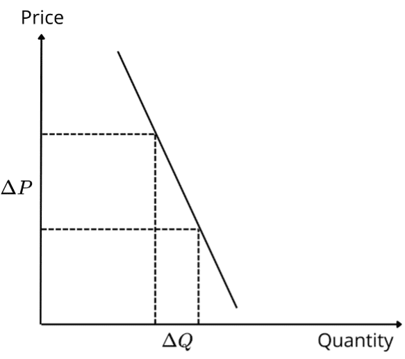
Thus, we speak of “elastic demand” if the result is greater than 1, and “inelastic demand” if it is less than 1. Conversely, if the result is exactly 1 —the relationship between demand and price is exactly proportional— we refer to “unit elasticity”. In Graph No. 1, different elasticity values can be observed along a straight-line demand curve. These concepts will be discussed in greater depth in section 4 on “Elastic and Inelastic Curves”.
Graph 1: Elasticity along a demand curve
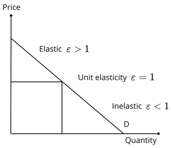
Source: Own elaboration
Similarly, supply price elasticity ( {\epsilon}_{P,o} ) measures the responsiveness of the quantity supplied of a good as a consequence of a change in its price, when all other factors that influence selling decisions remain unchanged (Parkin, 1990).
The price elasticity of supply is calculated using the following formula:
{\epsilon}_{P,o} = \frac{\Delta \% Q_{o}}{\Delta \% P}
Where “ \Delta \% Q_{o} ” represents the percentage change in the quantity supplied.
Considering that the quantity supplied of a good is generally positively related to its price, the price elasticity of supply is positive.
The cross-price elasticity of demand, or simply cross-elasticity of demand, measures the sensitivity of the quantity demanded of one good with respect to a change in the price of another good, when all other factors remain unchanged (Mankiw, 1997).
The cross elasticity of demand is calculated using the following formula:
{\epsilon}_{P,c} = \frac{\Delta \% Q_{d1}}{\Delta \% P_{2}}
Where “ \Delta \% Q_{d1} ” represents the percentage change in the quantity demanded of good 1; and “ \Delta \% P_{2} ” represents the percentage change in the price of good 2.
Unlike “common” demand elasticity (referred to as ‘own-price elasticity), which is shown in its absolute value, cross demand elasticity may be positive or negative depending on the relationship between the two goods under analysis (i.e., substitute goods or complementary goods).
Two goods are substitutes when an increase in the price of one leads to an increase in the demand for the other (in this case, there is a positive sign in the cross elasticity of demand). Intuitively, this happens because substitute goods satisfy similar needs (e.g., tea and coffee). So, if the price of coffee (good 2) increases, consumers will prefer to consume more tea (good 1) than coffee, and the quantity demanded for tea will increase. In conclusion, with substitute goods, cross elasticity of demand is positive: an increase in the price of good 2 generates an increase in the quantity demanded of good 1.
In contrast, two goods are complementary when an increase in the price of one leads to a decrease in the demand for the other. Generally, this occurs because complementary goods are used together (e.g., coffee and sugar). An increase in the price of coffee may lead people to choose to consume less sugar. In this case, the cross elasticity of demand is negative: an increase in the price of good 2 generates a reduction in the quantity demanded of good 1.
Income elasticity of demand ( {\epsilon}_{I,d} ) measures the sensitivity of the quantity demanded of a good in response to a change in consumer income, when all other factors remain unchanged (Mankiw, 1997).
Income elasticity of demand is calculated using the following formula:
{\epsilon}_{I,d} = \frac{\Delta \% Q_{d}}{\Delta \% I}
Where “ \Delta \% I ” represents the percentage change in consumer income.
According to the direction (positive or negative sign) of income elasticity of demand, goods can be normal goods or inferior goods.
In the case of normal goods, income elasticity of demand is positive. Intuitively, if consumer income increases, the quantity demanded of normal goods also increases, and vice versa (when a person’s income decreases, the demand for that good will decrease). It should be noted that most goods exhibit “normal” behavior, including luxury goods and basic needs (food or clothing).
On the other hand, inferior goods exhibit negative income demand elasticity: as consumer income increases, the quantity demanded of inferior goods tends to decrease, and vice versa. Low-cost fast food and low-quality clothing are examples of inferior goods.
To illustrate these concepts, let’s suppose we want to calculate the price elasticity of demand for a good, for which we have the following information:
Graph 2: Demand curve
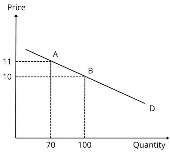
Source: Own elaboration
To calculate the elasticity between both points, it is necessary to get the data of the percentage changes in price and in quantity demanded.
Generically, the percentage change between two points is calculated by dividing the variation by the initial value, that is: \frac{Y_{2}-Y_{1}}{Y_{1}} \times 100 . Applying this to the price elasticity of demand formula we get the following:
{\epsilon}_{P,d} = \frac{(\frac{Q_{2}-Q_{1}}{Q_{1}}) \times 100}{(\frac{P_{2}-P_{1}}{P_{1}}) \times 100}
Where Q represents the quantity, P the price, and the subscripts “1” and “2” refer to the starting and ending points, respectively.
If point A is considered the starting point, the quantity and price experience percentage changes of -30% and 10%, respectively:
\Delta \% Q_{d} = (\frac{70-100}{100}) \times 100 = -30\%
\Delta \% P = (\frac{11-10}{10}) \times 100 = 10\%
Therefore, the price elasticity of demand is:
{\epsilon}_{P,d} = \frac{-30 \%}{10 \%} = |-3| = 3
However, if we calculate elasticity in the opposite direction, taking point B as our starting point, we obtain a different result:
\Delta \% Q_{d} = (\frac{100-70}{70}) \times 100 \approx 43\%
\Delta \% P = (\frac{10-11}{11}) \times 100 \approx -9\%
{\epsilon}_{P,d} = \frac{43 \%}{-9 \%} \approx |-4,7| = 4,7
The difference between both results is caused by the fact that percentage changes are calculated using a different base (the respective initial value).
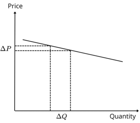
One way to resolve this discrepancy is to calculate percentage changes using as a base the “midpoint” between the initial and final values. That is:
{\epsilon}_{P,d} = \frac{(\frac{Q_{2}-Q_{1}}{(Q_{1}+Q_{2})/2}) \times 100}{(\frac{P_{2}-P_{1}}{(P_{1}+P_{2})/2}) \times 100}
With this methodology, the value of elasticity is the same in both directions:
{\epsilon}_{P,d} = \frac{\frac{100-70}{(100+70)/2}}{\frac{10-11}{(10+11)/2}} = \frac{\frac{70-100}{(100+70)/2}}{\frac{11-10}{(10+11)/2}} \approx |-3,7| = 3,7
For this reason, the midpoint method is considered a more accurate measure of elasticity between two points (Parkin, 1990).
The procedure for calculating other types of elasticities ( {\epsilon}_{P,o} , {\epsilon}_{I,d} , {\epsilon}_{P,c} ) is analogous, since only the variables under scrutiny change. For example, the formula to calculate the income elasticity of demand using the midpoint method is:
{\epsilon}_{I,d} = \frac{(\frac{Q_{2}-Q_{1}}{(Q_{1}+Q_{2})/2}) \times 100}{(\frac{I_{2}-I_{1}}{(I_{1}+I_{2})/2}) \times 100}
Where I represents consumer income.
Supply and demand curves can be classified according to their elasticity in relation to price.
The demand or supply for a good is said to be elastic when the elasticity is greater than 1 ( \epsilon >|1| ); that is, when it responds more than proportionally to a change in price. In the extreme case, when elasticity is infinite, the quantity demanded or supplied for a good is said to be perfectly elastic.
Graph No. 3 illustrates an elastic demand curve: a small change in price generates large variations in the quantity demanded.
Graph 3: Elastic demand
Source: Own elaboration
Graph No. 4 illustrates a perfectly elastic demand curve. In this context, the demand curve is represented by a horizontal line at price level, \bar{P} . For any price above \bar{P} , the quantity demanded is zero. When the price is exactly \bar{P} , the consumer is willing to purchase any quantity of the good. When the price is below \bar{P} , the quantity demanded is infinite.
Graph 4: Perfectly elastic demand curve
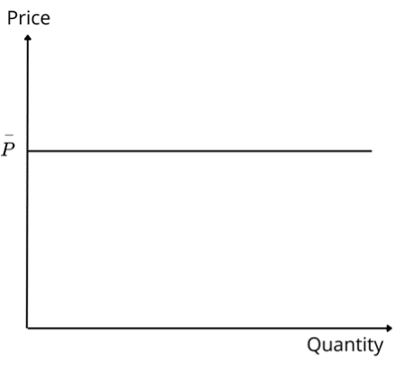
Source: Own elaboration
Conversely, the supply or demand for a good is considered inelastic when elasticity is less than 1 ( \epsilon <|1| ), which implies that the percentage change in quantity is less than the percentage change in price. When elasticity is equal to zero, the supply or demand curve is perfectly inelastic.
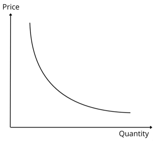
Graph No. 5 illustrates an inelastic demand curve: large variations in price have very little effect on the quantity demanded.
Graph 5: Inelastic demand
Source: Own elaboration
Graph No. 6 illustrates a perfectly inelastic demand curve. In this scenario, the quantity demanded is fixed ( \bar{Q} ), which implies that, at any price, the same quantity of the good is always demanded. For example, essential medicines tend to have perfectly inelastic or “very inelastic” demands, since people are willing to pay any price for a fixed quantity of the medicine (and when they are patented, they often lack substitutes).
Graph 6: Perfectly inelastic demand
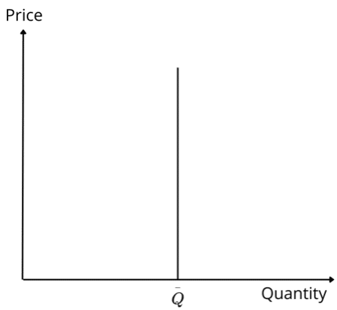
Source: Own elaboration
Finally, when elasticity is exactly 1 ( \epsilon =|1| ), quantity changes proportionally to price and is said to have unit elasticity.
Graph No. 7 illustrates a demand curve with unitary elasticity:
Graph 7: Unit elasticity demand
Source: Own elaboration
Goods vary significantly in their elasticities. In this section we study the factors which explain that the demand or supply for one good is more elastic than that of another.
Availability of substitutes
The more or better substitutes there are for a good, the greater its price elasticity of demand, since consumers can easily switch to other options if the price increases.
Luxury goods vs. necessities
Luxury goods tend to be more elastic than necessities. Specifically, luxuries are not essential for everyday life, so they can be easily discarded when prices rise. In contrast, necessities (e.g., basic food items) are difficult to replace, even if their prices increase considerably.
Proportion of income spent on the good
The greater the proportion of income spent on a good, the greater its price elasticity of demand. Consumers are more sensitive to the demand for these goods because a small change in their price can greatly affect their total spending.
Time horizon
Price elasticity of demand for a good will be greater the longer the time since the price change. A longer time horizon allows buyers to adapt their consumption habits and adjust to the new market conditions.
Nature of production
The easier it is to acquire the inputs needed to produce a good, the greater the supply price elasticity. In this sense, the availability of inputs makes it easier for producers to increase the quantity of a good supplied in response to a price increase. Availability of idle capacity and flexibility of production technology also improve producers’ ability to respond.
Time horizon
As in the case of the demand price elasticity, the price elasticity of supply for a good will be greater the longer the time elapsed since the price change. This occurs because, while production possibilities tend to be rigid in the short term, a sufficiently long time horizon allows companies to reorganize their production to adjust appropriately to new market conditions.
Elasticity is frequently used in the economic analysis of competition law cases. This tool provides valuable information for defining relevant markets, identifying competitors, assessing market power, and inferring competitive intensity, among other applications.
Below, we review two cases in Chile in which the concept of elasticity was applied.
On September 2, 2011, Quiñenco entered into an agreement to acquire, through its subsidiary Enex, all of the tangible and intangible assets of Terpel Chile. Both companies were involved in the distribution and sale of liquid fuels.
On November 10, 2011, the parties to the transaction filed a consultation to the Tribunal de Defensa de la Libre Competencia (TDLC), requesting that the institution clarify whether the acquisition complied with competition law rules (contained in Decree Law No. 211). The TDLC initiated non-contentious proceedings under case number NC 400-11/399-11 (accumulated cases), which included the participation of the Fiscalía Nacional Económica (FNE), trade associations, and other industry stakeholders.
Among the background information gathered for the investigation, Quiñenco presented an economic report entitled “Un análisis económico de los efectos competitivos de la compra de Terpel por Enex”, prepared by economists Alexander Galetovic, Ricardo Sanhueza, and Fernando Díaz. In order to assess the competitive intensity in the market analyzed, the authors estimated the price elasticity of demand faced by each of the service stations operated by Enex.
The report considered the estimated elasticities to be “high”: in some of the geographical zones under scrutiny, the minimum elasticity observed was 9.0, and in the Metropolitan Region, it was 11.6. According to these estimates, if any Enex service station slightly increased its prices, the quantity demanded would be drastically reduced. Thus, the authors interpreted these results as evidence that competitive intensity was high, stating that under these conditions, firms could not exercise market power. In line with the above, the economists concluded that the transaction analyzed did not pose any anti-competitive risks.
However, on April 26, 2011, the TDLC rejected the transaction, pointing to the existence of unilateral and coordinated risks that would not be offset by any of the efficiencies claimed by the Parties.
Thus, the Parties requested that the Supreme Court amend the ruling, declaring that the consulted transaction complied with competition law rules. On January 2, 2013, the Supreme Court upheld the appeal, approving the transaction subject to mitigation measures.
In particular, the Supreme Court denied the transaction would generate a significant reduction in competition, and added that, although the liquid fuel distribution market was concentrated and had oligopolistic traits, there was no concrete evidence to indicate that the merger would increase the risks of coordination.
On November 30, 2011, the FNE sued three chicken producers (Agrosuper, Ariztia, and Don Pollo) and the Chicken Producers Association (APA). These entities were accused of entering into a collusive agreement that limited chicken production, controlling the quantity produced and offered on the domestic market.
To assess the potential anti-competitive effects of the agreement, the FNE defined the relevant market as “the production, commercialization, and wholesale distribution of fresh chicken meat throughout the national territory”.
The companies argued that meat from other animals, such as pork and beef, should also be considered part of the relevant market. To support their position, these companies cited studies of cross-elasticity between chicken, pork and beef. These studies showed that the cross-elasticity of demand was in the range of 0.4-0.5. In effect, the estimation of cross-elasticities of demand with respect to chicken meat, having a positive sign (), showed a substitution relationship between the different types of meat.
However, the TDLC pointed out that the fact that two goods exhibit a degree of substitution is not sufficient to assert that both products belong to the same relevant market, and that other variables and methodologies must be considered in the analysis (Considering No. 24). Specifically, the TDLC considered various elements of demand that could refute the thesis of substitutability put forward by the poultry companies, such as consumer interest in purchasing a variety of products, the existence of discounts on other meats, and the possibility of freezing meat (allowing consumers to distribute their consumption among different meats over time).
Finally, the TDLC upheld the complaint and convicted the three companies and the APA of collusion in the production and allocation of quotas in the fresh chicken meat market between 1994 and 2010. The Supreme Court confirmed the ruling and increased the monetary penalty for the APA.
